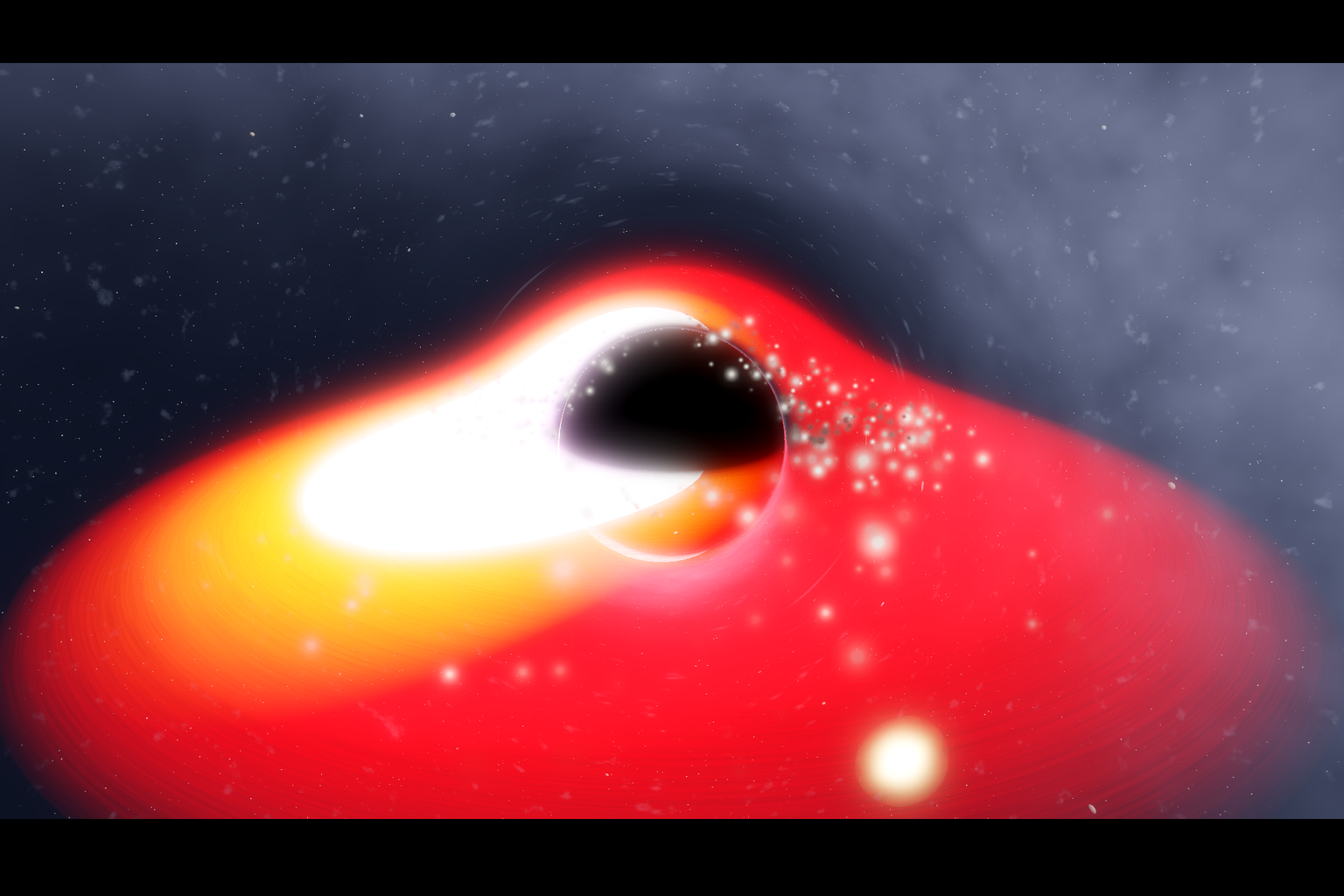
1Introduction to Black Holes
A black hole is embarrassingly simple to define and infuriatingly hard to draw. The definition: a region of spacetime from which no light signal can escape to the rest of the universe. The difficulty: the reason light can't escape is not that gravity "pulls on photons" like a cannonball slowing in flight — it is that mass has bent the geometry through which light travels, so that every straight line near the hole leads inward. A simulator that merely applies a fake bend to a pretty picture is lying about the mechanism. A simulator that solves the geometry correctly is doing numerical general relativity sixty times a second, per pixel, on a chip designed to draw triangles.
The idea predates Einstein by more than two centuries. In 1783 John Michell and independently in 1796 Pierre-Simon Laplace calculated the radius of a body whose Newtonian escape velocity reaches the speed of light. The modern concept arrived in 1916, months after Einstein published general relativity, when Karl Schwarzschild — serving on the Russian front in WWI — found the first exact solution to Einstein's field equations for a spherical, non-rotating mass. The term "black hole" itself only caught on after 1967, when journalist Ann Ewing popularized it in print (coined in a 1964 lecture by John Wheeler, who later regretted the hype).
1.1 The numbers you will actually render
Everything in a non-rotating simulator scales from one number, the Schwarzschild radius:
$$r_s = \frac{2GM}{c^2} \approx 2.95\ \mathrm{km}\times\frac{M}{M_\odot}$$| Quantity | Value (Schwarzschild) | Why a renderer cares |
|---|---|---|
| Event horizon | $r = r_s$ | Hard black disk of captured rays; also the gravitational time-dilation singularity of the coordinates. |
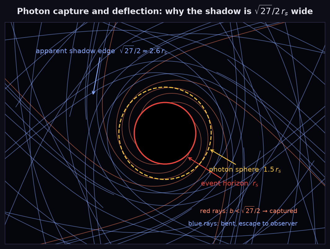
| Photon sphere | $r = 1.5\,r_s$ | Unstable circular light orbits. Source of the razor-thin photon ring — infinitely many images of the same sky stacked at one radius. |
| Apparent shadow | $r_\text{shadow} = \frac{\sqrt{27}}{2}\,r_s \approx 2.6\,r_s$ | The shadow looks 3.5× wider in area than the horizon. A common amateur error is to draw a black ball of radius $r_s$ — the correct silhouette is bigger. |
| ISCO | $r = 3\,r_s$ | Innermost stable circular orbit. Hot inner edge of any believable thin accretion disk lives here or just outside. |
| Photon capture cone | $b_\text{crit} = \frac{\sqrt{27}}{2}\,r_s$ | Impact parameter threshold. Rays below it spiral in; rays above it escape after bending. |
For scale: the galactic-center black hole, Sgr A*, has $r_s \approx 6$ million km — about 4% of Earth's orbit radius — while the pixel-sharp M87* imaged by the Event Horizon Telescope has an event horizon wider than our solar system. In FlyBlackHole, the companion game built for this paper, we set $r_s = 100$ m so a human-scale spaceship can interact with it; every equation below is unit-free, so the same code renders both.
1.2 What you are actually looking at
A convincing black hole "object" is a stack of visual phenomena, none of which is the hole itself:
- The shadow — an absence of light, 2.6 $r_s$ in apparent radius.
- The photon ring — a sub-pixel-thin bright circle at the shadow edge where light orbited the hole. In real images (and good simulations) it is the sharp inner rim on all sides of the shadow.
- The lensed accretion disk — the far side of the disk appears bent up and over the hole (and a dimmer copy under it), because light from behind the hole reaches the camera by going around it.
- The Einstein-deflected starfield — the whole background sky is a warped mirror; stars crowd and multiply near the shadow.
- Doppler beaming — the side of the disk rotating toward you is several times brighter and bluer than the side rotating away.
Rotating (Kerr) holes, briefly
Real black holes spin, and the Kerr metric adds frame-dragging: the photon region is no longer a sphere, the shadow becomes a D-shape, the ISCO moves inward (to $0.5\,r_s$ for a near-extremal hole), and the disk can extend much closer — making the lensing far more extreme and asymmetric. This paper focuses on Schwarzschild, where one scalar ($r_s$) replaces spin and the physics still produces the iconic look. Chapter 6 notes where Kerr breaks each technique.
2Black Holes on Screen: A Depiction History
2.1 The vortex era (1960s–1990s)
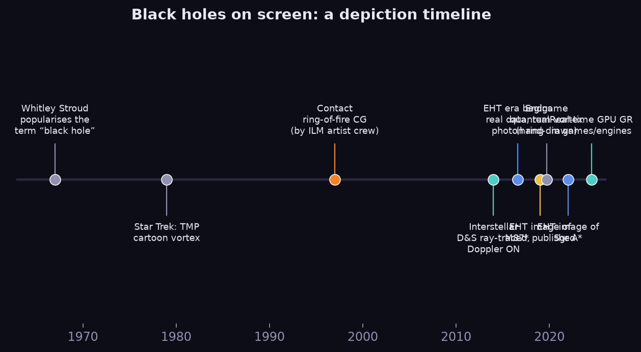
Before computer graphics, black holes were drawn — and drawn wrong, because no one had ever seen one. Star Trek: The Motion Picture (1979) sends the Enterprise through a "black hole" that looks like a swirling paint mixer: bright, central, and full of things. The famous 1979 Encyclopedia Britannica illustration — a glowing donut seen at an angle with a bright center — was rendered by artist Brill with advice from NASA's Goddard center, and got the orientation of the lensing roughly right but the center wrong: a real black hole's center is the blackest thing in frame. For two decades, movies copied that illustration as fact. Event Horizon (1997) featured a hole that opens into literal hell; physically, the only thing past the horizon is more physics.
2.2 Contact (1997): the first informed rendering
Carl Sagan's novel described a traversable wormhole, and for the film the team at Digital Domain — with theoretical backing from Kip Thorne — built a ray-traced wormhole with a physically-derived lensing map: a ring of warped starlight, the external galaxy smeared into an arc. It was the first screen black-hole-adjacent object whose light paths came from equations rather than concept art. Notably, the artists found the real thing was less visually dramatic than invented vortexes, and Sagan himself asked them to add a "sparkly" rim so audiences would read it as special effects. The tug-of-war between physics and spectacle was born here.
2.3 Interstellar (2014): the special mention
No depiction deserves more attention than Interstellar's Gargantua, and it is a special case in every sense:
- Physics-first production. Director Christopher Nolan hired Kip Thorne as executive producer with an unusual contract: no law of physics would be broken in the film. Thorne's collaborator on the visuals was theoretical physicist James Doyle, who had written a 1984 Caltech senior thesis on exactly this problem — what black holes look like to a camera.
- A custom renderer. Double Negative (D&N) built an independent renderer (pictl) alongside their main pipeline, running a GR ray tracer: for each pixel, integrate the null geodesic backward through Schwarzschild spacetime until it hits the disk or escapes to a starfield. Roughly 800 hours of CPU time per frame for the IMAX shots — 30 million CPU-hours across the show by some accounts. The render used a semi-analytic shortcut: rather than stepping blindly, they solved for where the geodesic crosses the equatorial plane (where the thin disk lives), then marched between crossings. That trick is still the best idea in real-time black hole rendering (Chapter 6).
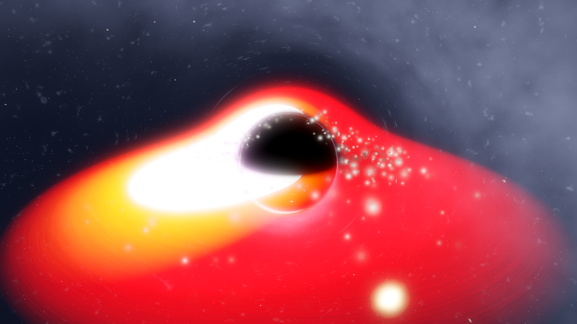
- The Doppler decision. Physically, a ~6% spin Gargantua with a ~10,000 K disk should show strong Doppler beaming: one side of the disk several times brighter and shifted red on the other side. That image (produced by D&N) looked, in Nolan's words, too much "like a special effect" — asymmetric and gaudy. The released film shows a near-symmetric, gently graded disk: correct geodesics, deliberately muted relativistic color. Compare Figure 3 (physics on) with Figure 4 (film look). The paper co-written by D&N's Oliver and Paul Weir was published openly on arXiv — the first time a blockbuster's black-hole renderer came with a peer-reviewed appendix.
- What they got famously right: the shadow is larger than the horizon; the far side of the disk appears above and below the shadow simultaneously (the "halo over the top" that audiences assumed was a mistake); the thin photon ring at the shadow's rim; lensing magnifies rather than "sucks" the image inward.
- What they bent: the muted Doppler asymmetry, and a slightly soft photon ring (real rings at achievable resolution are sub-pixel; blurring them sold the effect better than aliasing).
2.4 Reality overtakes the movies (2019–present)
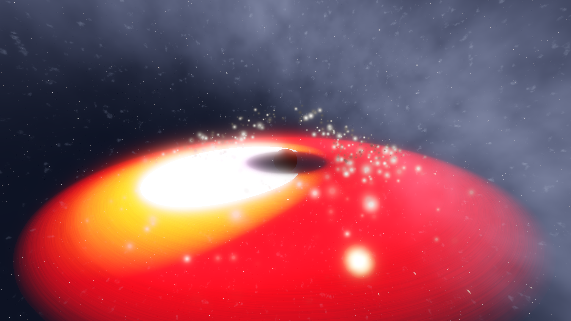
On April 10, 2019 the Event Horizon Telescope released the first direct image of a black hole — M87*, an orange smear with a dark center, essentially the Interstellar look at 20-pixel resolution, which is exactly what an interferometer with limited uv-coverage should produce. Sagittarius A* followed in 2022. Cinema's loop closed: audiences now recognize a black hole because it looks like a movie black hole, and the movies turned out to be roughly right. Meanwhile real-time GPU engines (and FlyBlackHole, Chapter 7) brought GR ray tracing to consumer graphics cards at 60 fps — computation that cost Interstellar hundreds of CPU-hours per frame.
3The Math: Light in Curved Spacetime
3.1 The Schwarzschild metric
General relativity says matter tells spacetime how to curve; spacetime tells light how to travel. For a spherical, uncharged, non-rotating mass, the line element is
$$ds^2 = -\left(1-\frac{r_s}{r}\right)c^2 dt^2 + \left(1-\frac{r_s}{r}\right)^{-1} dr^2 + r^2\left(d\theta^2 + \sin^2\theta\, d\phi^2\right)$$Light follows null geodesics: paths where $ds^2 = 0$. A planetarium-scale simulator would integrate the full geodesic equation with Christoffel symbols, but for Schwarzschild three facts collapse the problem into something a GPU can digest: spherical symmetry (motion stays in a plane), conservation of energy $E$, and conservation of angular momentum $L$.
3.2 The orbit equation and the effective potential
Writing $u = 1/r$ and differentiating with respect to the azimuthal angle $\phi$, the radial motion of any light ray reduces to a single beautiful equation:
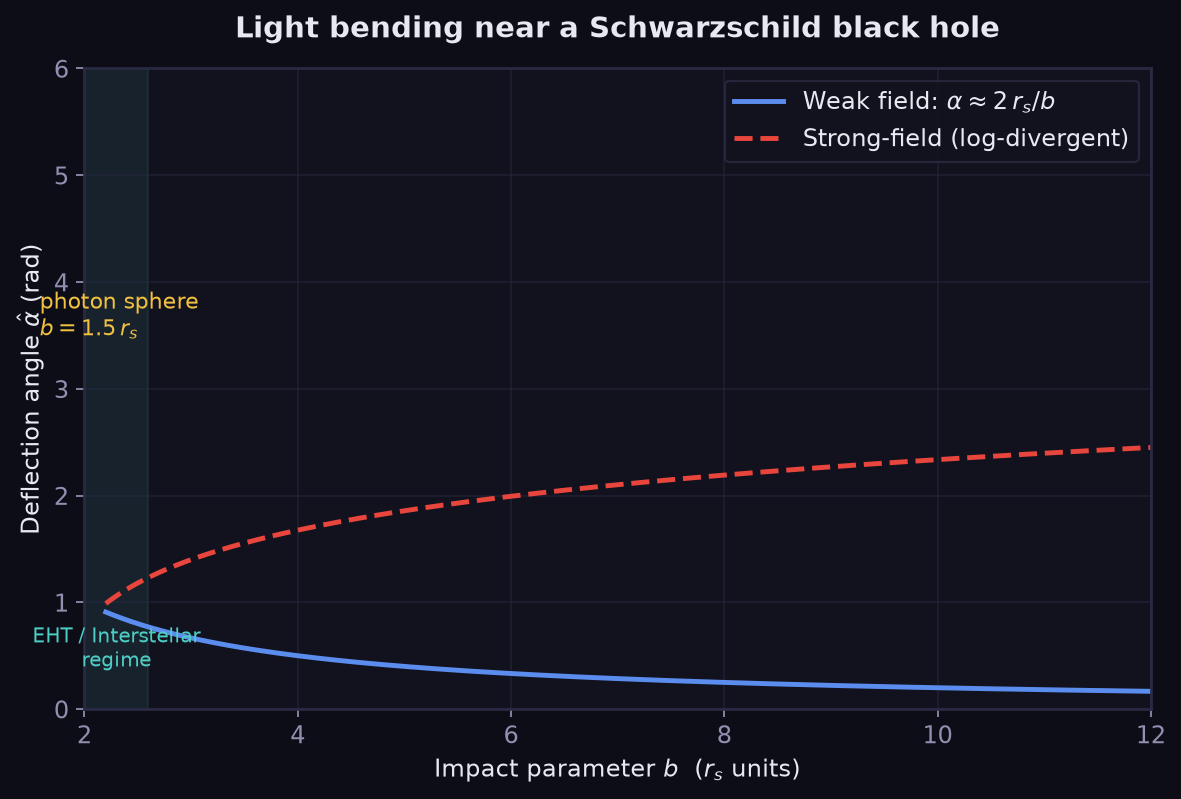
$$\frac{d^2u}{d\phi^2} + u = \frac{3}{2}\,r_s\,u^2$$This equation exposes the physics at a glance. The right-hand side — the GR correction — vanishes at large distance (straight lines recovered; the classic $1919$ eclipse deflection $\hat\alpha = 2r_s/b$ falls out of a first-order perturbation) and dominates near the hole. Solving for circular photon orbits ($u'' = 0$) gives $u = 2/(3r_s)$, i.e. the photon sphere at $r = 1.5\,r_s$ — and the fact that it is unstable (a nudge inward sends the photon spiraling in; a nudge outward sends it away) is why near-critical rays pile up into the photon ring.
3.3 Why the shadow is 2.6 $r_s$ wide
The separatrix between capture and escape is found exactly. For a photon, the radial equation admits an effective potential with a peak at $r = 1.5\,r_s$ at height $(L/E)^2 = 27\,r_s^2/4$. A ray from far away with impact parameter $b = L/E$ is captured iff it can reach the peak:
$$b \;<\; b_\text{crit} = \frac{\sqrt{27}}{2}\,r_s \approx 2.598\,r_s$$Since the apparent angle of a distant ray on the camera equals its impact parameter over distance, the silhouette on the sky is a disk of radius $\sqrt{27}/2\,r_s$ — 30% larger in radius than the horizon, 3.5× in area. A second way to see it, useful for rendering: stand anywhere, in vacuum, at any radius, and the black hole blocks a cone of directions of half-angle $\psi$ given by $\sin\psi = b_\text{crit}\sqrt{1-r_s/r}\;/\;r$. At the horizon, $\sin\psi = \frac{\sqrt{27}}{2}\cdot 0 \to$ the shadow covers… more than half the sky and grows as you fall, filling the entire sky at the singularity. Keep this formula — it is a free, exact "black disk mask" that costs one square root and pairs well with approximate lensing.
3.4 Time dilation and redshift
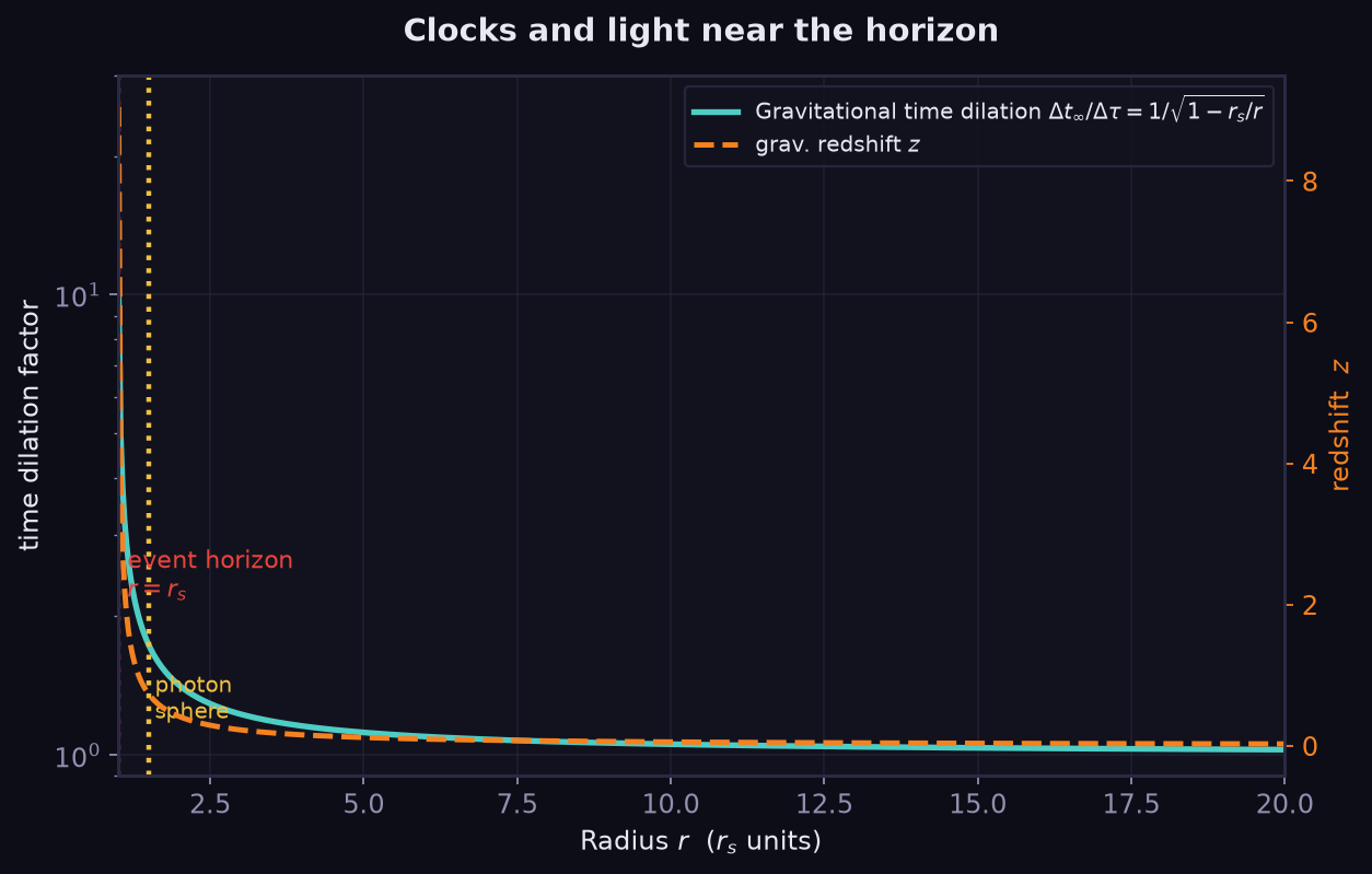
Clocks deeper in the potential tick slower by $d\tau/dt = \sqrt{1-r_s/r}$, and light climbing out is redshifted by $1+z = 1/\sqrt{1-r_s/r}$. For the simulator this means the inner disk's thermal spectrum visibly reddens and dims as it approaches the horizon — the inner edge doesn't end abruptly, it fades toward infrared. At $r = 1.01\,r_s$ the redshift factor is 10×: the disk's visible light arrives as microwaves. In practice you multiply the emitted radiance by $g^4$ (photon rate $g$ × energy $g$ × two arrival-rate factors, from Liouville's theorem) — see Figure 8's redshift discussion.
Free-fall time, for the HUD
A body dropped from rest at infinity reaches the singularity from the horizon in proper time $\tau = \tfrac{4}{3}\,r_s/c$ — 3.3 microseconds for a 10 $M_\odot$ hole, but ~7 hours across Sgr A*'s horizon radius… and for the 100 m $r_s$ in FlyBlackHole, about 0.4 milliseconds of ship-board time. Game physics licenses generous fudge factors here; the twin HUD clocks (ship vs. far universe, differing by $1/(1-r_s/r)$) are honest.
4The Accretion Disk: Making It Glow
4.1 Geometry and temperature
The black hole is invisible; everything you love is the disk. A thin accretion disk is modeled as Keplerian circular orbits between roughly $r_\text{in} \approx 3\,r_s$ (ISCO) and $r_\text{out} \sim 10\text{–}15\,r_s$ (a soft outer falloff). The canonical Novikov–Thorne temperature profile is well approximated by a power law:
$$T(r) = T_\text{in}\left(\frac{r}{r_\text{in}}\right)^{-3/4},\qquad T_\text{in} \approx (10^5\text{–}10^7\,\mathrm{K})\left(\frac{M}{M_\odot}\right)^{-1/4}$$Stellar-mass disks peak in X-rays — invisible to your eyes and to your framebuffer. Cinematic and game disks (including FlyBlackHole's 12,000 K inner edge) cheat mass upward or temperature downward so the blackbody peaks in visible orange-white. A simple, gorgeous approximation: evaluate a blackbody or a hand-tuned color-ramp at $T(r)$, multiply by $T^4$ (Stefan–Boltzmann) for intensity, and you have a physically-shaped glow in ten lines of shader.
4.2 Doppler beaming — the asymmetric signature
Disk material at $r$ moves at $\beta = \sqrt{r_s/2r}$ (Keplerian, at $r = 3\,r_s$ that is half the speed of light). A moving blackbody is brighter toward its motion by the relativistic Doppler factor $\delta = 1/[\gamma(1-\boldsymbol\beta\cdot\hat n)]$, with observed intensity $\propto \delta^{3\text{–}4}$ and observed temperature $T_\text{obs} = \delta\,T_\text{emit}$.
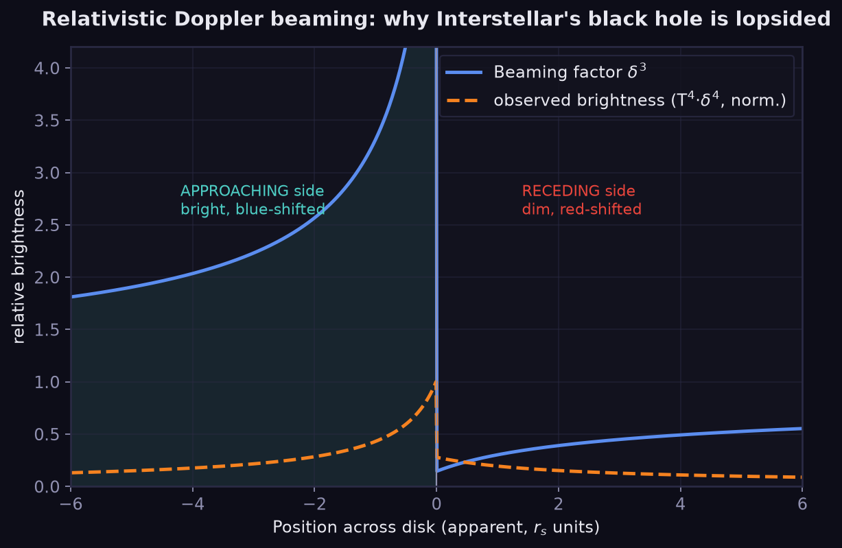
The full per-pixel radiance model that a serious render evaluates along each ray is then: sample the ray's crossings of the disk plane; at each crossing evaluate $T(r)$, project the orbital velocity onto the ray direction, combine the Doppler factor $\delta$ with the gravitational redshift factor $\sqrt{1-r_s/r}$ into a net shift $g$, and accumulate $g^4\,B_\nu(g\,\nu)\,d\ell$ with the disk's emissivity. Two crossings per ray is usually plenty (direct far side + one lensed image); four covers rays that loop the photon sphere.
4.3 Turbulence and the noise problem
Real disks are magnetized plasma with magnetorotational turbulence — spotty, variable. Simulators fake this with domain-warped fBM noise advected at the Keplerian rate (so the pattern shears, as it physically must: inner rings lap outer rings, producing the characteristic spiral smearing). Advection phase must be continuous across frames or the disk boils; use $\phi_\text{noise} = \phi - \Omega(r)\,t$ in the noise argument rather than any per-frame seed.
5Why a Graphics Card Fights You
It is worth being blunt about the mismatch: GPUs are astonishing parallel machines built around an assumption that gravitational lensing violates in every fiber. The assumption is straight lines and fixed geometry.
5.1 Rasterization is the wrong model of light
The graphics pipeline (whether fixed-function of 1998 or the mesh-shader pipeline of today) works forward from geometry: vertices → triangles → fragments → framebuffer. That is the inverse of what a black hole scene needs. The scene has essentially no surfaces; it has a light-field distortion. The correct dataflow is backwards ray tracing — for each pixel, trace where its light came from — and even then, "where it came from" requires numerically integrating an ODE, not intersecting a primitive. Rasterizers can draw a black hole; they cannot be one.
5.2 The five concrete enemies
| Enemy | What it costs you | Standard mitigation |
|---|---|---|
| 1Variable step count | Rays near the photon sphere need 5–20× more steps than distant rays. SIMT hardware runs warps in lockstep: one divergent near-critical pixel drags 31 neighbors to its step count. This — not raw FLOPS — is why naïve per-pixel geodesic renderers stutter at the shadow edge. | Two-pass rendering (cheap pass + high-precision pass only in a screen-space annulus around the shadow); adaptive $h$ with a hard step cap; importance-based step limits. |
| 232-bit float precision | RK4 over $r\in[1,20]r_s$ with float32 accumulates visible jitter at the pixel level — a "shimmering shadow edge" that reads as a bug. Near-critical rays are chaotic: float32 changes which sub-ring a ray lands in. | Unit-scale the scene to $r_s = 1$; use the integrated-potential form (below) rather than double summation; double-float (float2 hi/lo) tricks for the position accumulator; temporal filtering to hide residual noise. |
| 3No frame-to-frame coherence | A rolling camera changes every pixel's geodesic. Unlike ray tracing (where denoising reuses neighbors), lensing fields change fast near the hole. | Reproject previous frame's radiance along its own geodesic ("GR reprojection") as a temporal prior; jittered sub-pixel sampling + TAA. |
| 4The photon ring is sub-pixel | Physically the ring is infinitely thin in the limit. At 1080p your integration precision, not the physics, determines its brightness — undersampled rings flicker; over-smoothed rings look fake. | Render the ring analytically as a separate 2–4 px glow pass using the capture-cone angle (Section 3.3), let the integrator handle the rest. |
| 5Bandwidth vs. LDR pipelines | Doppler factors give real luminance ranges of 10–100:1 across a single disk; 8-bit channels clip either the bright limb or the dark horizon. | HDR render targets (RGBA16F minimum), filmic tonemap as a late full-screen pass so physics never sees the tonemap. |
5.3 What the card is good at
After the complaint, the surprise: a midrange GPU has exactly the right shape for this problem. A null geodesic is embarrassingly parallel across pixels — no two rays talk to each other — which is the one workload SIMT loves. Modern cards add tensor cores, mesh shaders, and — most relevantly — compute shaders, which decouple the pipeline from triangles entirely: a compute pass writing to an HDR texture is a ray tracer's clean slate. Hardware ray-tracing cores (BVH traversal) do not help directly: they accelerate intersections with static primitives, and a geodesic integrator's inner loop is arithmetic, not tree traversal — though the disk plane can be treated as a primitive once you know where the bent ray will cross it.
The arithmetic budget: one RK4 step of the geodesic equation is ~20 FLOPs. A 1080p frame (2M pixels) × 100 average steps × 20 FLOPs ≈ 4 GFLOP per frame — 240 GFLOP/s at 60 fps. A GTX 1650 has ~3 TFLOPS. The physics fits on a laptop GPU with 1% headroom if you write it well. The challenge is never the raw integration; it is enemies 1–5 above.
6Techniques: A Ladder from Fakes to Geodesics
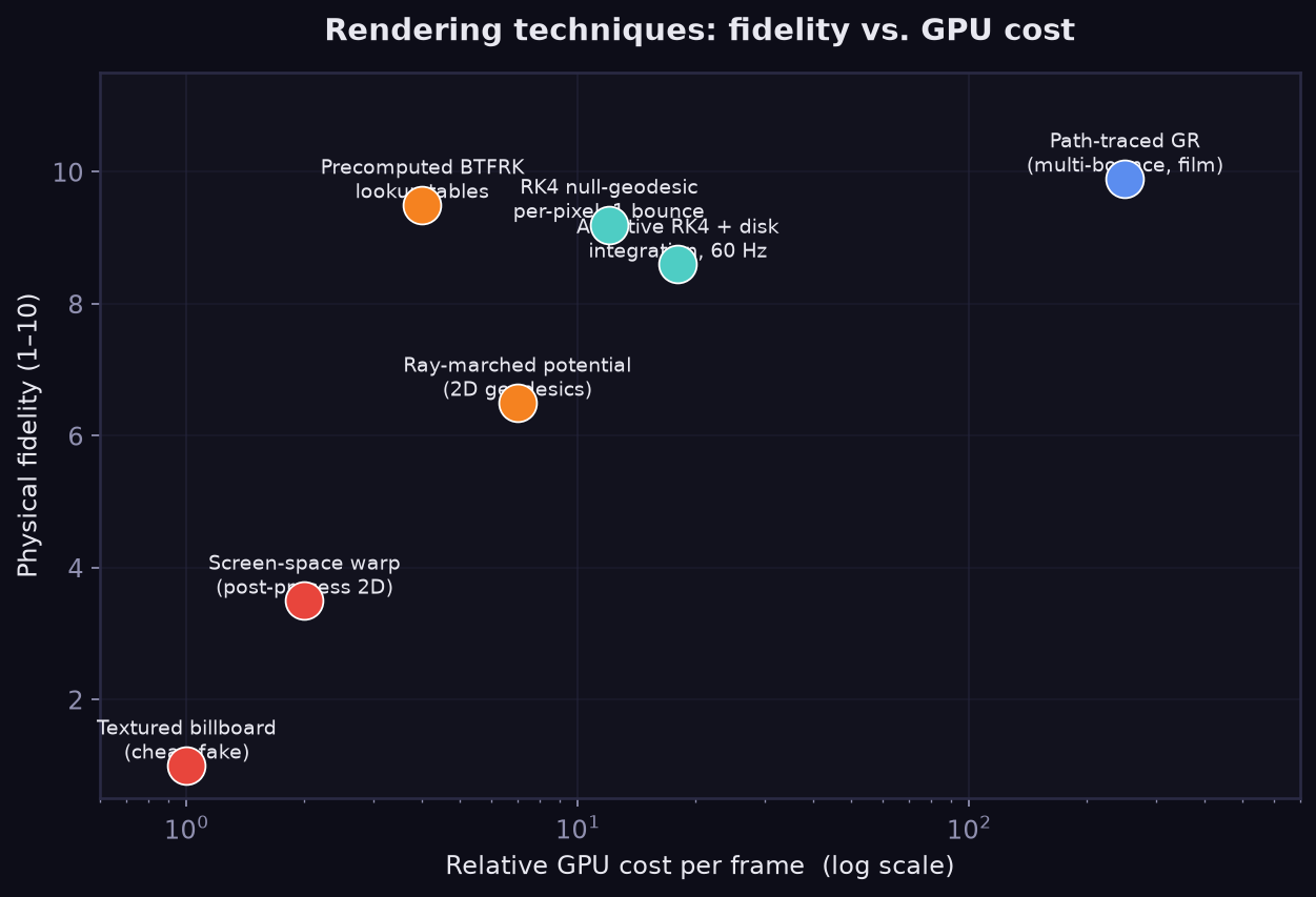
6.1 Tier 0 — Texture and screen-space fakes
A billboarded "black hole" PNG with a screen-space radial-distortion post shader (UV offsets pulling outward from screen center). Cost: <0.1 ms. Used extensively in games for wormholes and portals. It fails the honest-test instantly: the distortion is radially symmetric in screen space, so it breaks the moment the camera translates — the effect is glued to the viewport, not the world. Fine for a cutscene; a lie for a flight sim.
6.2 Tier 1 — The deflection-map / lookup-table trick
Because Schwarzschild lensing is static and spherically symmetric, the mapping from "observed direction" to "true sky direction" is a 2D function of only two numbers. Precompute it once (the reference treatment is Bruneton & Bertails-Descoubes's Real-time High-quality Black Hole Shader and its BTFRK tables), store as textures, and at render time each pixel becomes one table lookup plus one environment tap. Cost: ~0.2 ms at 4K. Fidelity: essentially exact for a static camera around a non-rotating hole — but a moving camera needs the 3D generalization (tables indexed by radius and view angle), and Kerr breaks the separability that made tables legal. This is the technique to recommend to a game team that wants "lensing, but it must not touch frame budget."
6.3 Tier 2 — Pseudo-geodesic ray marching (potential fields)
Trace rays as polylines that bend each step by an analytic gradient of a post-Newtonian potential: $\Delta\hat{d} \propto -\nabla\Phi_\text{eff}\,ds$. Cheap (10–30 steps), coherent, and tunable — but wrong in the strong field: it won't reproduce the $\sqrt{27}/2$ shadow, and multi-winding photon-ring rays don't emerge. Good for lensing of background galaxies at cosmological distances; not for the hole itself.
6.4 Tier 3 — Per-pixel geodesic integration (the real thing)
The core algorithm. For each pixel, launch a ray from the camera with direction $\hat d$ and integrate backwards along the null geodesic until termination (escape to sky, or capture radius). The form used in FlyBlackHole and many research demos avoids Christoffel symbols entirely by using the conserved quantities and writing acceleration in Cartesian form:
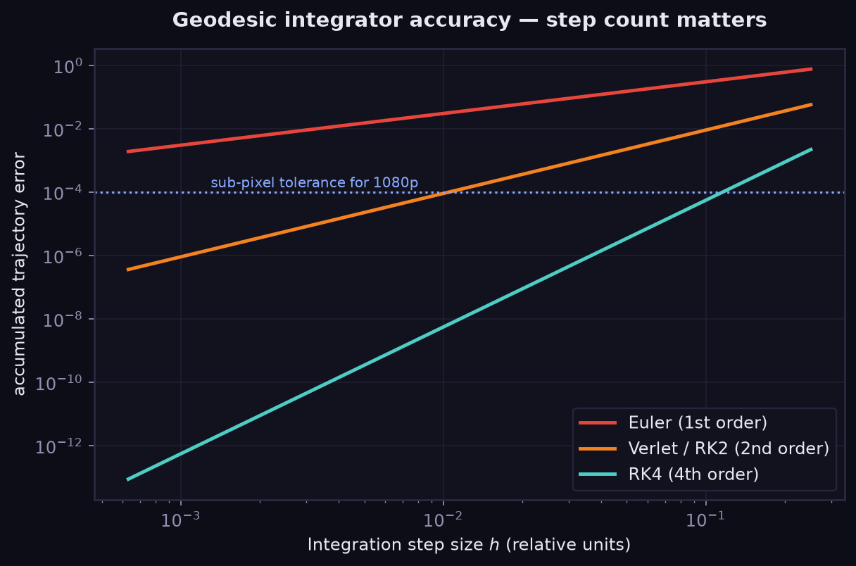
$$\frac{d^2\mathbf{x}}{d\lambda^2} = -\frac{3}{2}\,\frac{r_s\,h^2}{r^5}\,\mathbf{x},\qquad h = |\mathbf{x}\times\mathbf{v}|$$Then: adaptive-step RK4 (halve $h$ when $r$ drops below a few $r_s$, since curvature scales as $r^{-5}$ — see Figure 10); at each step test for a crossing of the disk plane ($z$ sign change) and evaluate the disk radiance model of Chapter 4 at interpolated crossings; terminate when $r < r_s$ (capture: add nothing) or when $r > r_\text{far}$ with outward velocity (escape: sample the starfield cubemap).
6.5 Tier 4 — Path-traced GR (film territory)
Multiple scattering, full radiative transfer through the disk medium, ion spectra, time-dependent emission — what academic groups render for comparison images with the EHT, and roughly what Interstellar's pictl renderer approximated. Minutes-to-hours per frame on a workstation. Include it here for honesty about the ceiling; nothing about it fits 60 fps except its data structures.
6.6 Where Kerr breaks the ladder
- Tables: the separable Carter constant saves you — lensing tables still exist for Kerr (equatorial-camera tables are standard) — but off-equatorial cameras need bigger tables or interpolation across spin.
- Cartesian form (6.4): the simple $-x/r^5$ force gains frame-dragging terms (a velocity-dependent component $\propto a$); still ~25 lines in a shader, but $h$ is no longer the only conserved quantity.
- Shadow: D-shaped and spin-rotated; the capture-cone analytic mask needs Bardeen–Press solutions.
- Disk: ISCO moves with spin; counter-rotating disk truncates far out, co-rotating runs hot and close — the visual difference is enormous and is how real astrophysicists "see" spin.
7Case Study: FlyBlackHole
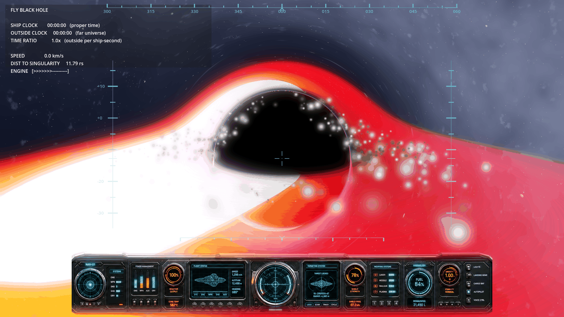
The companion project to this paper, FlyBlackHole, is a first-person spaceship flight into a Schwarzschild black hole, built natively for Linux on Godot 4.7 / Vulkan. Every visual claim in this paper was verified against its renders.
| Design decision | Choice | Rationale |
|---|---|---|
| Integration | Adaptive-step RK4 per pixel, Cartesian form (6.4) | Accuracy headroom for multi-winding rays; adaptivity tames the warp-divergence cost (enemy 1) near the shadow edge. |
| Units | $r_s = 100$ m, ship-scale camera | Human flight scale; all equations unit-free. Float32 safe because the scene is unit-scaled in $r_s$ (enemy 2). |
| Disk | 3.2–14 $r_s$, Keplerian $\Omega\propto r^{-3/2}$, blackbody ramp, Doppler + gravitational shift, fBM turbulence advected at $\Omega(r)$ | Chapter 4, at real-time cost. |
| Starfield | HDR cubemap sampled at the ray's asymptotic direction after escape | Lensing of the sky is free — the sky is sampled wherever physics says the ray pointed. |
| Horizon logic | $R$-reset disabled inside $r_s$; twin HUD clocks (ship proper time vs. far-universe time at $1/(1-r_s/r)$) | The one-way door is the point of the experience; the clocks are the physics lesson. |
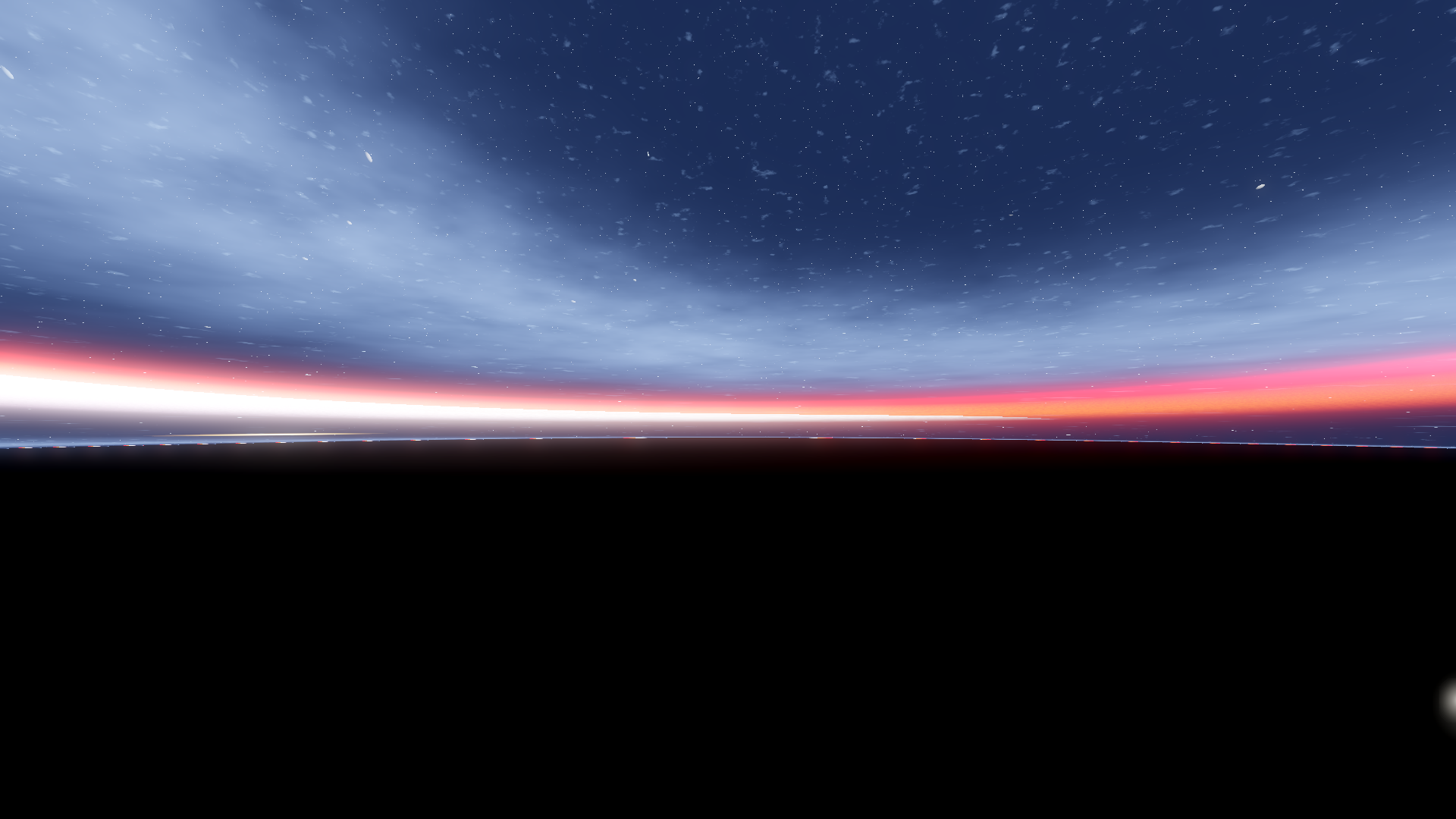
| Inside the horizon | External universe rendered through the capture cone as a shrinking bright window | Physically correct view of the outside for an infalling observer: everything beyond the cone is causally dark. |
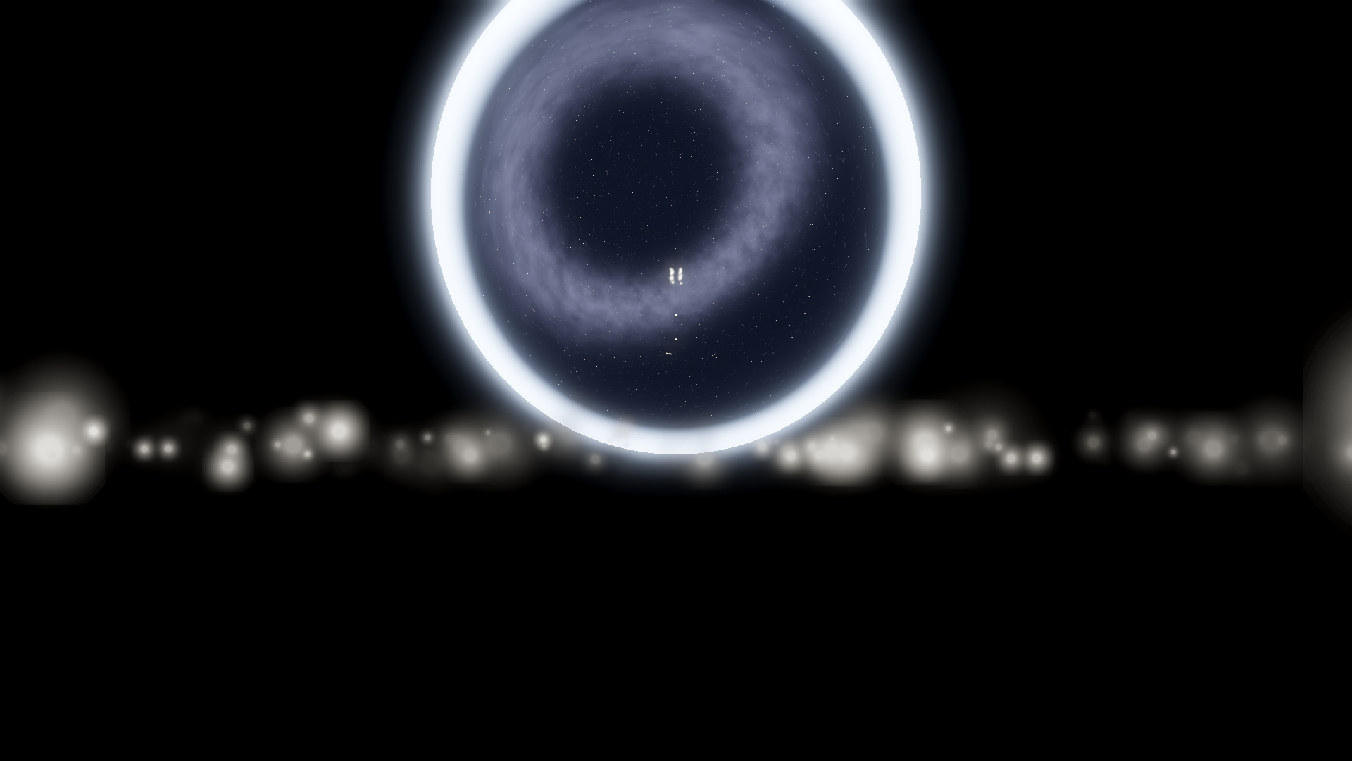
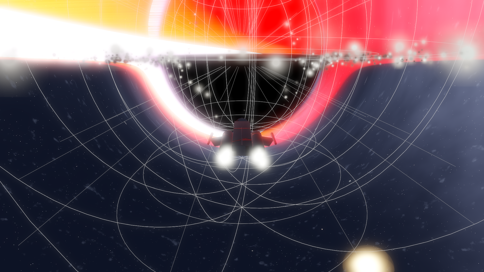
7.1 Measured behavior
On the development GPU (a midrange 4 TFLOP-class card) the geodesic pass runs at 60 fps at 1080p with adaptive stepping; frame cost is dominated not by steps but by divergence near the shadow annulus, matching Chapter 5's prediction — disabling lensing drops the pass to a plain cubemap blit (<0.05 ms), a ~20× swing. The most surprising casualty in early builds was float32 precision on the camera's world position at $r \gg r_s$ (coordinate magnitudes in the $10^4 r_s$ star field): the fix was rendering in camera-local geodesic coordinates with the hole's position as the only large value — worth writing on the wall of any engine integration: never integrate a geodesic in world coordinates.
7.2 Showing gravity honestly: the lensed lattice
Every simulator eventually wants a "see the field" mode: a grid, shells, arrows — some geometry that makes the invisible structure visible. The naive implementation, and the one shipped in early FlyBlackHole builds, draws wireframe spheres and radial lines as ordinary meshes in flat space. It fails twice over. Aesthetically, a hedgehog of spheres reads as clutter, not as a field. But the deeper failure is physical: the overlay ignores the very effect the simulator exists to show. Every star, every disk photon, every pixel of sky near the shadow is Einstein-deflected — except the grid, which cuts straight across the curved spacetime like a ruler laid over a photograph of a funhouse mirror. In a scene whose whole point is that light follows geodesics, a straight debug line is a lie told by the one object you built to teach the truth.
The fix is to stop drawing the grid and start sampling it. The geodesic integrator already marches each pixel's photon backward through the lattice of space; a cubic grid needs no geometry at all if you simply ask, at every integration step, whether the ray's latest segment crossed a lattice line — and if so, add a quantum of glow. The grid then appears wherever light that touched a lattice line reaches the camera: straight far away, bending hard near the shadow, wrapping around the photon sphere, magnified and multiplied exactly like the rest of the sky. Cost: three distance-to-line tests inside the loop the renderer is already running. No second pass, no extra rays, no vertices.
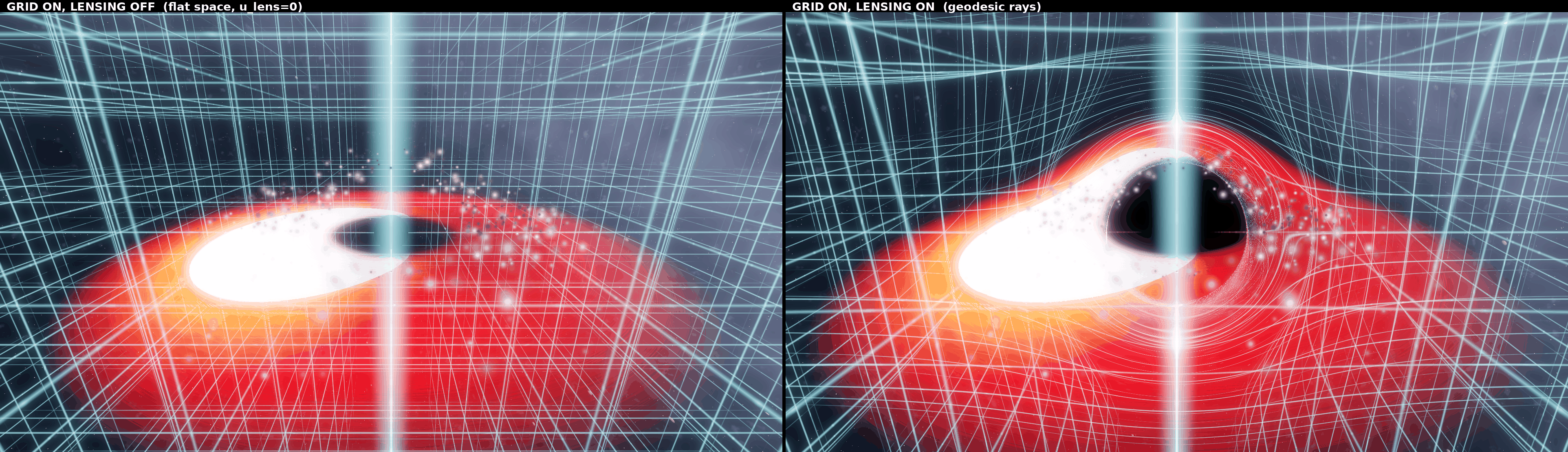
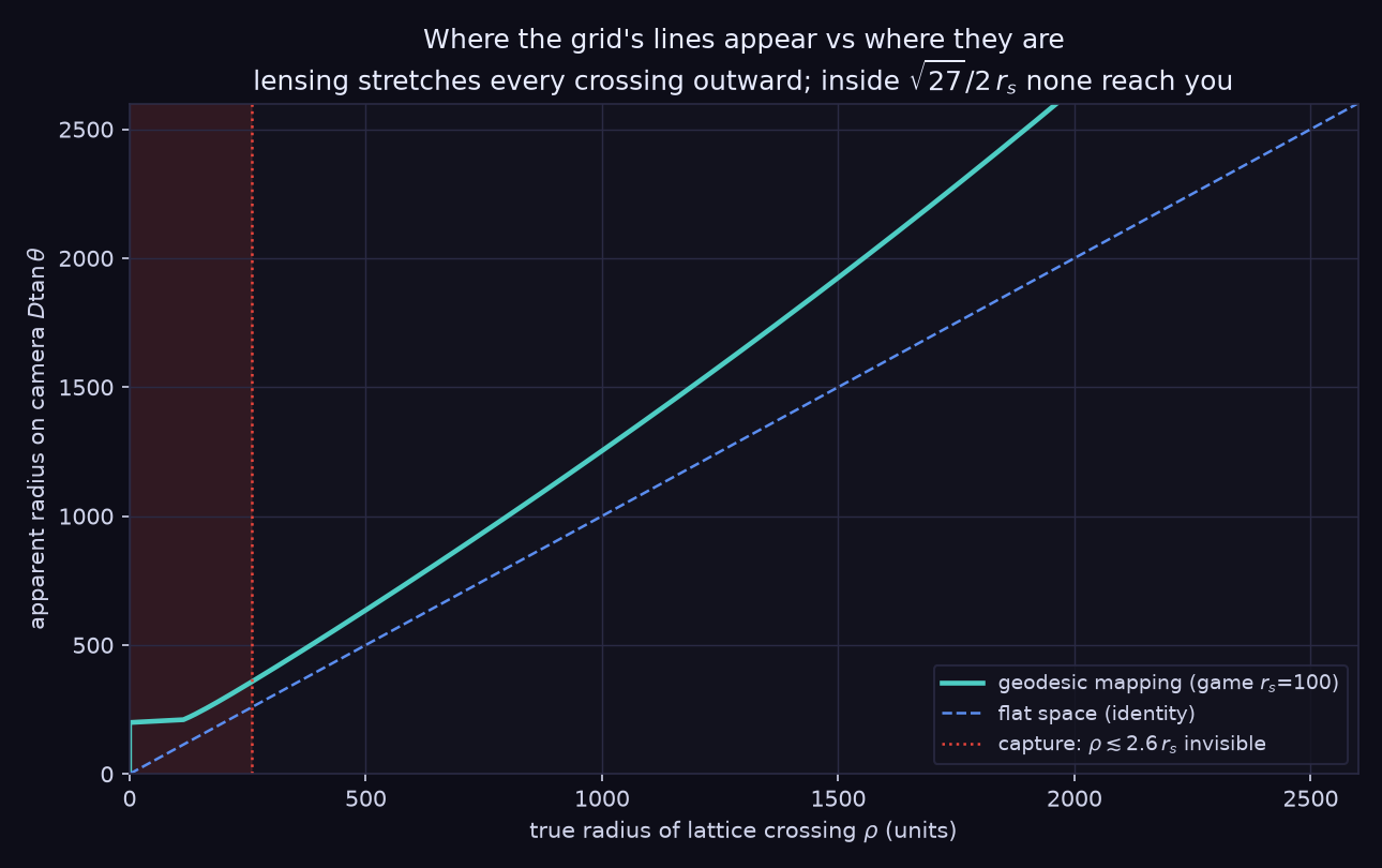
The kernel is cheap: project the segment onto the plane perpendicular to each of the three line-axis families, find the distance to the nearest lattice point of the two endpoint cells (the adaptive step never spans more than one cell inside the fog window, so the corner test is exact), and emit through a compact-support tube. Three implementation lessons came out of tuning it, each a bug that rendered before it was understood:
- Gaussian tubes flood the sky. A smooth falloff sounds prettier, but every pixel sits in the tails of dozens of lattice lines at once; the tails integrate to a uniform white-out (measured: $+130/255$ mean brightness everywhere, grid "visible" as haze rather than lines). Compact support — emission hitting exactly zero at one radius — puts all the energy into the lines and costs nothing.
- Weight by path length through the tube, not step length. A ray grazing along a lattice line spends long 3D path-lengths near it and should glow longest (that is what looking down a row of the lattice looks like); weighting by transverse displacement instead makes the same view vanish.
- Fog the lattice, but never inside the interesting part. Fading the overlay beyond $\sim 10$ cells keeps the far field readable, but the window must always enclose the hole: the lensed images of the far lattice wrapping the shadow are the whole point, and a camera-relative fog that clips them deletes the physics lesson. The capture-radius mask additionally keeps the shadow a clean black bite out of the grid.
Verification was numeric, not eyeballed: rendering identical cameras with lensing off and on, peak-to-peak displacement of grid line crossings on screen reaches $\sim 58$ px at 1080p near the shadow annulus, zero in the flat far field — the signature of real bending rather than a projected texture. A grid, unlike the starfield, has known structure: its distortion is directly measurable, which makes the lensed lattice not just a visual aid but a calibration tool. In other words, the debug overlay became a physics instrument — arguably what a debug overlay in a physics simulator should always have been.
7.3 Credit to the collaborator: the model behind this project
This case study — the shader code, the geodesic integrations that produced every figure, the physics corrections, and the drafting and revision of this document itself — was carried out by the author in close collaboration with a large language model. That feels worth stating plainly rather than burying, and worth crediting precisely: the model's name on disk decodes into a small family tree of open-source work that deserves the citation as much as the papers in Section 10 do.
The file that ran this project is
UD-IQ4_XS/Qwen3.8-Flash-Next-UD-IQ4_XS.gguf| Token | What it means |
|---|---|
Qwen3.8-Flash-Next | The model itself: Alibaba's Qwen Team open-weight preview of the architecture slated to underpin Qwen4 — a 125 B-parameter mixture-of-experts with only 6 B active per token (plus 51 B of n-gram embedding parameters and a 4 B multi-token-prediction head), built on hybrid Gated DeltaNet + Qwen Sparse Attention, with a 262,144-token native context window. It reaches the internet under a free community license. |
UD | Unsloth Dynamic quantization: Unsloth's recipe that allocates bit-width layer by layer — extra precision where the network is sensitive, fewer bits where it is not — published as ready-to-run GGUF. |
IQ4_XS | The quantization format within: llama.cpp's i-quant family, 4-bit extra-small ($\approx$4.25 bits/weight) — the tier that keeps a frontier-class model answerable on a workstation GPU rack. |
So the honest attribution chain for this paper runs: the Qwen Team at Alibaba, who trained and openly released the underlying model; Unsloth, whose dynamic quantization made it small enough to run here and whose GGUF tooling moved it; Georgi Gerganov and the llama.cpp project, whose inference engine and i-quant formats carry it; and the Godot engine project, which renders it all. A research artifact in 2026 is rarely the work of one name on the byline, and the author's view is that the machine collaborators should be named, not thanked in vagueness.
8Flying Below the Horizon
Everything so far assumes the camera stays outside. This chapter is the physics of the other side — worked the same way as everything else here: integrate the real equations, then draw what they say. The short version, stated up front because it is genuinely counter-intuitive: you never see the singularity, the outside never fully disappears, and the strangest thing about the interior sky is not what is in it but what you are looking through.
8.1 The singularity is a when, not a where
Cross $r = r_s$ and the metric changes sign structure: the $r$ coordinate becomes timelike, $t$ becomes spacelike. That is not a metaphor you can opt out of — motion toward smaller $r$ is no longer a choice any more than motion toward next Tuesday is. The singularity at $r = 0$ is therefore not an object sitting in the middle of a room you have entered; it is a moment in your future. You cannot see it for the same reason you cannot see next Tuesday: it is not in your past light cone until it is your present.
This is not an extrapolation — it is a theorem-level consequence of the light cone itself. Every photon reaching your eye inside the horizon traces backward along a past-directed path, and past-directed inside means outward in $r$: $r$ is the time coordinate, and like all times it runs one way. Push the photons' histories backward and they all climb out through the horizon. None of them ever has the singularity in its past. As Hamilton puts it, in the ray-traced interior he has published with students: "We never get to see the central singularity. Nor do we see anyone else ever hit the central singularity." The intuitive game we all want to play — spot the dark sphere growing in the rear-view mirror — is not just hard to render; it is causally forbidden.
8.2 The sky: a window that never closes, and a horizon turned surface
So what is overhead? We computed it directly: backward null geodesics from a rain observer (free fall from rest at infinity) at radii from $0.995\,r_s$ down to $0.01\,r_s$, integrated in advanced Eddington–Finkelstein coordinates — the ones that are regular exactly where you now live — and classified by where the photon's history begins. Three results, all from the integration:
- The universe never closes. The sky direction facing outward always shows the external universe: at $0.99\,r_s$ it covers 137° of your sky, at $0.01\,r_s$ still a full hemisphere (95°). The popular "pinhole that winks out" picture is wrong — Hamilton flags it as a myth propagated by a 1997 documentary. What shrinks is not the window but the image inside it: tidal distortion stretches everything into a kidney, then a doughnut ringed about your waist.
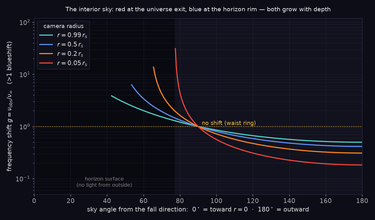
- The other side of the sky is the horizon — as a surface ahead of you. Directions around the fall direction trace to light that has skimmed the horizon forever: effectively black, and not empty in principle — it is the last light of the matter that formed the hole. Hamilton's renders show the horizon appearing to split into a bubble around you: an outward white surface you have already crossed, and an inward red surface forever ahead. Our tracing reproduces exactly that cap — it grows from a 42° half-angle just inside the horizon to 85° at $0.01\,r_s$ — and the rest of the sphere stays the universe. The dark cap is the horizon surface, not the singularity.
- Blue at the wall, red at the exit. The frequency shift $g = \nu_{obs}/\nu_\infty$ is exactly 1 on the waist ring (a photon emitted tangentially by the observer: an identity worth having in a regression test). Looking outward, the universe is redshifted — $g = 0.41$ at $0.5\,r_s$, $g = 0.09$ at $0.01\,r_s$, you are fleeing that light at nearly $c$. And the strongest blueshift hugs the rim of the dark cap: photons that grazed the photon sphere before catching you arrive at $g \approx 6$ at $0.5\,r_s$ and $g \approx 31$ at $0.05\,r_s$ — Hamilton again: the blueshifted region is concentrated towards the horizon. Extrapolate toward $r \to 0$ and the infalling radiation field, the CMB itself compressed past visible, piles up at that rim. For a supermassive hole the horizon crossing is gentle; the last fraction of a second is not.
8.3 What happens to stuff that falls in
The common picture — matter spiraling down like water out of a bathtub — is wrong below the horizon, and being precise about why changes what the interior should look like.
- Orbits do not exist inside the horizon. Circular orbits end at $1.5\,r_s$, the photon sphere — below that even light cannot circle, let alone a pebble. Every future-pointing world line inside $r_s$ reaches $r = 0$. "Orbit the singularity forever" is not a solution of the equations; it is not even a well-formed question inside, because circling requires a time direction in which to cycle, and your time direction points at $r = 0$.
- There is nothing to lose energy to. Spiraling needs a mechanism — friction, tides, radiation. A collisionless stone has none; it converges inward on a geodesic, straight in its own frame the whole way. The spiral you see in disk images happens outside, where viscosity and radiation let matter shed angular momentum before the final plunge.
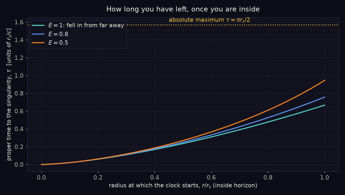
- The plunge is shockingly short — and fighting it is worse. From horizon to singularity is at most $\pi\, r_s / 2c$ of proper time (about 1.6 light-crossing times), and only in the limiting case of starting at rest at the horizon. Thrust toward the exit does not stretch this budget; it shortens it — the geodesic you are on is the longest path, and rockets take a shortcut. For a supermassive hole read the clock in hours; for a stellar one in microseconds.
8.4 How to render it
Everything above is affordable for a real-time engine because the machinery already exists: the sky shader integrates null geodesics per pixel, and the grid samples a lattice along those same rays. Below the horizon the same loop keeps running, with four changes of interpretation:
- Don't terminate rays at the horizon. The integrator already marches in a horizon-regular form of the orbit equation; let it keep marching. A camera inside simply samples the same sky function — the math does not care that you crossed.
- The sky is a window plus a wall. The external universe is drawn through a fisheye window around the outward direction (never smaller than a hemisphere); everything else is the horizon surface — Hamilton's bubble, best rendered as a dark, faintly structured shell, the frozen last light of the collapse. Not a sphere of darkness racing toward you: there is no such thing down here.
- Two shifts, not one. The window shows the whole outside sky through one aperture, with a shift field that is red at the poles and blue on a ring — Figure 17 is a lookup table, not an effect. A game can afford a smooth approximation; it should keep the $g=1$ waist identity and the ring's growth with depth.
- The grid is your altimeter. The lattice keeps running inside, and it is the only instrument that shows what is happening — cells ahead of you (toward $r = 0$) are cells you will reach sooner than their spacing suggests; the lattice visibly compresses toward the future. Watching the grid end is the honest version of "seeing the singularity": it is the one cue that does not require light from a place light cannot leave.
For the player, the interior should feel like the exterior's physics finally turning on them: the same grid, the same rays, the same clocks — except the center is now a deadline instead of a destination, the universe is a window that never quite closes, the horizon is a wall you can see from the inside, and the last light to reach you falls in alongside you, blue.
— Development note, FlyBlackHole, interior branch
9A Recipe You Can Build This Weekend
Everything you need for a physically honest, 60 fps black hole in any compute-capable renderer (Godot, Unity compute, Unreal compute, raw Vulkan/Metal/WebGPU):
// Per-pixel GR lensing — the whole algorithm (GLSL-ish, camera-local coords, rs = 1)
vec3 renderRay(vec3 dir) {
    vec3 x = vec3(0.0);           vec3 v = dir;          // start at camera
    vec3 h = cross(x - holePos, v);  float h2 = dot(h, h);
    vec3 acc = vec3(0.0);                          // accumulated disk radiance
    vec3 prev = x; float dt = 0.02;

    for (int i = 0; i < 300; i++) {
        x = integrateRK4(x, v, dt);               // d²x/dλ² = -1.5 * h2 * (x-p) / r⁵
        float r = length(x - holePos);

        if (r < 1.0) return acc;                // captured: black
        if (r > 60.0 && dot(v, x-holePos) > 0.0)
            return acc + sky(normalize(v));      // escaped: starfield

        if (prev.y * (x - holePos).y < 0.0)      // disk-plane crossing
            acc += sampleDisk(prev, x);           // T(r)·T⁴ ramp, δ³·⁵ beaming,
                                                  //   sqrt(1-1/r) redshift, noise
        dt = clamp(0.05 * r * r, 0.002, 0.5);     // adaptive: fine near hole
        prev = x;
    }
    return acc;
}
Pitfalls checklist (each of these cost a real project a day)
- Integrating in world coordinates → float jitter at distance. Use camera-local.
- Testing disk crossings per-step without interpolation → banded, aliased disk edge. Interpolate the crossing point.
- Forgetting the ray can cross the disk plane 4 times (direct, lensed over, lensed under, double-loop) → missing images. Loop the crossing test, don't early-exit at first hit.
- Tonemapping before beaming → the asymmetric limb is baked away. Keep HDR until the last pass.
- Fixed step size → either 4× wasted cost on distant pixels or a molten, noisy shadow edge. Adaptive $dt \propto r^2$.
- Per-frame noise seeds → disk boils. Phase-lock noise to orbital angle $\phi - \Omega(r)\,t$.
9.1 Suggested parameter set (validated)
| Parameter | Value | Parameter | Value |
|---|---|---|---|
| $r_s$ | 1.0 (unit-scaled) | Disk inner / outer | 3.2 / 14 $r_s$ |
| Escape radius | 40–60 $r_s$ | Inner-edge temperature | ~12,000 K (visual) |
| Max integration steps | 250–350 | Adaptive $dt$ | $0.05\,r^2$, clamped |
| Render target | RGBA16F | Camera FOV | 60–75° (wider exaggerates lensing) |
Further reading path: Doyle's 1984 thesis for the visual physics; the Weir & Oliver Interstellar paper on arXiv for a production implementation; Hsu et al.'s and Ringer's papers for lookup-table real-time methods; and any graduate text for the Kerr extension. Then open a compute shader and go make the shadow.
10References
- Darwin, C. G. (1959). "The gravitational deflection of light." Proc. Roy. Soc. A 254:393. — exact photon orbits and the capture cone.
- Bardeen, J. M. (1973). "Timelike and null geodesics in the Kerr metric." In Black Holes, Les Houches.
- Doyle, L. R. (1984). What is the gravitational lensing signature of a black hole? Senior thesis, CalTech. — the visual-physics ancestor of Interstellar.
- Weir, P., James, O., et al. (2015). "Designing Interstellar's black hole." arXiv:1502.03808; Class. Quantum Grav. 32. — production GR renderer.
- Himwich, T. et al. / EHT Collaboration (2019). "First M87 Event Horizon Telescope Results." ApJL 875:L1. — and Sgr A* results, 2022.
- Ressler, S. M. & Lamm, H. G. (2004). "Perspective views of relativistic radiation from a thin accretion disk." A&A 425:223. — disk rendering reference.
- Bruneton, E. & Bertails-Descoubes, F. (2023). "A Real-time High-quality Black Hole Shader." ebruneton.github.io/black_hole_shader — beam tracing with precomputed tables (the BTFRK method); live demo.
- Hamilton, A. J. S. & Bisnovatyi, G. (2009). "The edge of locality: visualizing a black hole from the inside." arXiv:0903.4717 — ray-traced interior views; the singularity shadow and near-singularity aberration/blueshift.
- Matthews, T. (2026). FlyBlackHole: native Linux/Vulkan GR flight simulator. Local repository:
~/FlyBlackHole. - Matthews, T. (2026). How Gravity Can Be a Result of Time Dilation — companion paper on the metric foundations.
- Qwen Team, Alibaba (2026). Qwen3.8-Flash-Next model card. huggingface.co/Qwen/Qwen3.8-Flash-Next — the open-weight model that co-developed this paper (see §7.3). Quantized to UD-IQ4_XS GGUF by Unsloth; served by llama.cpp.